Hi all! In the previous post I had discussed about how to search satellite imagery and other spatio temporal data using STAC in QGIS. Honestly it's very convenient to find a satellite imagery for a certain time in a certain area from multiple domains using STAC. We only need an URL link and the STAC tool will search for collections of data that available. Seamlessly it will enhancing and fostering the use of spatio temporal data in a GIS application to solve a real world problem.
More than that, the use of STAC to find any related spatio temporal data can be more powerful combining with a programming language like Python. It's not only about searching a specific data but also elaborate other spatial computation and analysis in a row.
The question is: How to implement STAC in Python? In this tutorial we'll get through it. This post will explain step by step approach how to use STAC in Python from searching data, display it and do analysis for the data. Keep reading!
Installing Libraries
We start this tutorial by importing some required libraries. For this
tutorial we need some libraries such as pystac-client, odc-stac, and matplotlib. Make sure you have the libraries, if you don't please install it first. For the installation you can use pip or conda depends on your environment.
1 2 3 | from pystac_client import Client from odc.stac import load import matplotlib.pyplot as plt |
Searching for Images/Assets with PySTAC
After import libraries, let's open a STAC with the URL: https://earth-search.aws.element84.com/v1 with the following code. Then we call all the collections with get_collections() method.
1 2 3 4 5 | client = Client.open("https://earth-search.aws.element84.com/v1") collections=list(client.get_collections()) number_collections=len(collections) print(f"{number_collections} collections") print(collections) |
If the collections variable is printed, we'll get result like this:
8 collections
[<CollectionClient id=cop-dem-glo-30>,
<CollectionClient id=naip>,
<CollectionClient id=sentinel-2-l2a>,
<CollectionClient id=sentinel-2-l1c>,
<CollectionClient id=cop-dem-glo-90>,
<CollectionClient id=landsat-c2-l2>,
<CollectionClient id=sentinel-1-grd>,
<CollectionClient id=sentinel-2-c1-l2a>]
The collections result return as a list. Then we can simply count the number of collections using the len function.
Now let's take sentinel-2-l2a collection. Define a boundary extent in the bbox variable and define a date range. Using those parameters do searching in the collection using client.search() method. Last two lines in the following code will print the item's id and percentage of cloud coverage.
1 2 3 4 5 6 7 | collection = "sentinel-2-l2a" bbox = [34.2201,31.1394,34.6694,31.6493]# min lon,lat, max lon, lat date="2023-12-01/2023-12-31" search = client.search(collections=[collection], bbox=bbox, datetime=date) print(f"{search.matched()} items found") for item in search.items(): print(item.id,":",item.properties['eo:cloud_cover']) |
Running the code we'll get the following result.
14 items found
S2B_36RXV_20231231_0_L2A : 1.321937
S2B_36SXA_20231231_0_L2A : 16.668269
S2A_36RXV_20231226_0_L2A : 0.003849
S2A_36SXA_20231226_0_L2A : 0.006606
S2B_36RXV_20231221_0_L2A : 100
S2B_36SXA_20231221_0_L2A : 100
S2A_36RXV_20231216_0_L2A : 48.060358
S2A_36SXA_20231216_0_L2A : 88.949937
S2B_36RXV_20231211_0_L2A : 9.257196
S2B_36SXA_20231211_0_L2A : 4.992877
S2A_36RXV_20231206_0_L2A : 25.865424
S2A_36SXA_20231206_0_L2A : 72.468609
S2B_36RXV_20231201_0_L2A : 1.460705
S2B_36SXA_20231201_0_L2A : 6.149376
From the result we know that the item with id S2A_36RXV_20231226_0_L2A has the lowest cloud coverage 0.003849%. We can use this item to work on. But it will be better if we can filter the result to select the lowest cloud coverage. The next code is used for this purpose.
1 2 | selected_item=min(search.items(),key=lambda item: item.properties["eo:cloud_cover"]) print(selected_item.id, selected_item.properties["eo:cloud_cover"]) |
We have a collection item, now let's find out what assets are available in it. To get all available assets the assets.items() method is used. Then using it's key and and title properties we print the result.
1 2 3 | assets=selected_item.assets.items() for key,title in assets: print(key,'|',title.title) |
Below is the sample result from the code.
aot | Aerosol optical thickness (AOT)
blue | Blue (band 2) - 10m
coastal | Coastal aerosol (band 1) - 60m
granule_metadata | None
green | Green (band 3) - 10m
nir | NIR 1 (band 8) - 10m
nir08 | NIR 2 (band 8A) - 20m
nir09 | NIR 3 (band 9) - 60m
red | Red (band 4) - 10m
rededge1 | Red edge 1 (band 5) - 20m
rededge2 | Red edge 2 (band 6) - 20m
rededge3 | Red edge 3 (band 7) - 20m
Preview/Plot The Image Using PySTAC
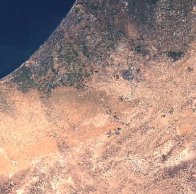
Assets are all available data within an item. We can select an asset and do something on it. But firstly let's see the scene using the thumbnail asset.
1 2 | from IPython.display import Image Image(url=selected_item.assets["thumbnail"].href, width=500) |
 |
| Figure 1. Image Preview |
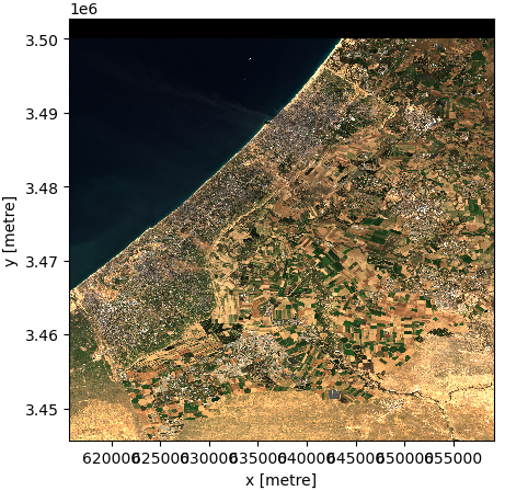
That's the preview for the whole scene. But how to view to the area of interest within the defined boundary area? For that we need to load the raw data using the load class from odc-stat module. I suggest not to load all the bands cause it will take time, it would be better to load only bands that are required. In this case I loaded four bands as you can see in the selected_bands list variable.
1 2 3 4 | selected_bands = ["nir", "red","green","blue"] data = load([selected_item], bands=selected_bands, bbox=bbox).isel(time=0) fig, ax = plt.subplots(figsize=(10, 10)) data[["red", "green", "blue"]].to_array().plot.imshow(robust=True, ax=ax) |
In the line 3-4, here comes code to display the image for the respected area. I want to view the natural color with bands combination red-green-blue. Figure 2 shows the plot of the image.
 |
| Figure 2. Natural Color Image |
NDVI Calculation Using PySTAC
So far, we have done searching data and view it in a plot. Now let's do a computation by doing a NDVI calculation. For NDVI calculation we need two bands: Red and Near Infrared band. For that we assign for each band with red and nir and perform NDVI calculation using the formula as in line 3 in the following code.
1 2 3 4 5 6 | red = data["red"].astype("float") nir = data["nir"].astype("float") ndvi = (nir - red) / (nir + red) fig, ax = plt.subplots(figsize=(7, 7)) ndvi.plot.imshow(ax=ax, cmap="Greens") |
Lastly let's view the result by plotting using the rest of the code.
 |
| Figure 3. NDVI Image |
This tutorial covers the essentials of using PySTAC. Throughout this tutorial, we've learned how to connect with a data provider, access its collections, and retrieve available items. We've also explored filtering Sentinel images to identify those with the lowest cloud coverage, plotting the images, and calculating the NDVI.
We hope this tutorial has provided you with a solid starting point for utilizing PySTAC. There's a wealth of additional functionality to explore with PySTAC, so be sure to visit the PySTAC website for further details. Thank you for reading!
Anyway I provide the code in a notebook based on request. If you're interested, please make your request here.