Heatmap Calculation Tutorial Using Kernel Density Estimation (KDE) Algorithm

Kernel Density Estimation (KDE) Overview

The previous post had discussed about Kernel Density Estimation (KDE) in creating a heatmap in QGIS. It explained about background and conceptual approach how KDE is applied for a heatmap production. This post will give a tutorial and example how to calculate a density value estimation around a point dataset. We will go step  by step, so hopefully this tutorial could give you a clear understanding how to do a density calculation using KDE.

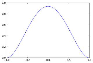
As explained before in the previous post, there are some KDE shapes which are using to construct a Probability Density Function (PDF) in order to estimate a density at a location to a reference point. In this tutorial, we will use quartic kernel shape. The quartic kernel shape has a function as in equation 1, with the shape of the kernel can be seen in figure 1. If a density value also considered a weight (W), a constant (K) and Intensity (I), then the function become as in equation 2. In this case we assume W=K=I=1. Therefore we will use equation 1 through out this example.

Equation 1. Quartic KDE function

Equation 2. Quartic KDE function with KWI

Figure 1. Quartic kernel shape

Kernel Density Estimation (KDE) Basic Calculation Example

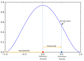
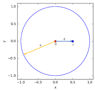
Using the kernel, then we will calculate an estimation density value at a location from a reference point. Figure 2 shows more detail about the quartic kernel shape and some properties such as bandwidth (h), reference point (O), estimation point (z) and the distance (d) from reference point to estimation point. Moreover figure 3 shows how it looks like in a space.

Figure 2. Quadratic Kernel Shape and related properties

Figure 3. KDE properties is space

Our goal is to find the density value at z. Knowing the distance (in this example 0.5), then we can calculate the density value using equation 1 as follow.

It is quite simple, isn't it? So we can calculate a density at any point within the bandwidth radius. When a point reaches the bandwidth radius (equal to 1) the density value will be 0, and we do not consider any point outside the bandwidth radius.

Kernel Density Estimation (KDE): More Complex Calculation Example

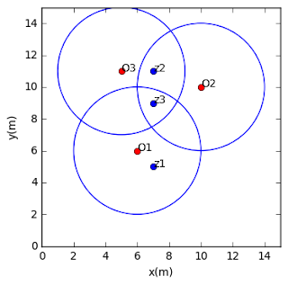
The example above shows the basic concept in estimating a density at a location from a reference point. Now let's see a more complex example. Figure 4, consist of 3 points data with coordinates O1(6,6)m, O2(10,10)m, O3(5,11)m. Next we want to compute the density estimation value at point z1(7,5)m, z2(7,11)m and z3(7,9)m. The kernel radius is 4 m.

Figure 4. Three points dataset and three estimation points

Before we do calculation, observe that z2 is in intersection area between O2 and O3 bandwidth radius and z3 is in intersection of all reference points radius. When a point lies in an intersection radius we have to sum up all density value from each reference point, then the density function becomes as in equation 3.

Equation 3. Summation of Quartic KDE function

 Now, let's do the calculation. Firstly we compute the density at z1, therefore we have to compute the distance O1-z1, with equation 3.

Equation 3. Formula to calculate distance between two points

 Then the distance O1-z1:

 

Great, we just need to use the computed distance, and done! But wait, it can't be like that. The distance can't be used right away. Why? The quartic kernel density function that we're using is in standardize form. It means the bandwidth radius has a fix number as 1. So we have to divide the computed distance with the actual kernel bandwidth (in this case is 4 m). 1.41/4=0.35. Thus the density at z1:

Next we compute the z2. Because z2 is in intersection of O2 and O3, first we calculate the distance of z2 to O2 and O3, then compute the density of z2 from each reference point and sum up the both result. The calculation can be seen as follow:

Lastly for z3:

In this tutorial we just calculated density for some points around the dataset. In a real case, the algorithm will calculate the density for a whole dataset area. For this we have to specify the size of output pixel. The calculation then will take place on each pixel. As the pixel size gets smaller, will produce a smoother result. But on the other hand, will require more resources for computation. Hopefully you could get a robust understanding how a heatmap is created using KDE. You can create a heatmap in QGIS using QGIS heatmap plugin. If you are interested to see how to apply this algorithm in Python see this post (How to Create Heatmap in Python from Scratch)    

 Geoanalytics