Heatmap is a nice visualization method to display event density or occurrence. Heatmap is also used in clustering points where more points in an area will have higher value compare to less point in the same area. Therefore, with a heatmap we can see a concentration of event's occurrence. For example criminal events in a city can be visualized in a heatmap, so one knows how the crime events spread around the city. Such map is commonly called a crime map.
To create a heatmap is quite easy and straight forward. There are many software and tools that can be used to produce a heatmap like QGIS, ArcGIS, Crimestat,
Google table fusion, etc. We just need to upload point dataset, setting some parameters and the result will come up. But the purpose of this post is not just to produce a heatmap with some clicks. But more than that to explore and trying to get more understanding what is going on behind the screen for data and parameters that have been specified. In another term, how the algorithm is working in producing a heatmap.
QGIS is an open source GIS software that can be used to produce a heatmap from a set of data point with
Heatmap Plugin. The plugin is using Kernel Density Estimation algorithm for creating a heatmap. Because of that I will discuss how this algorithm(Kernel Density Estimation) is applied to process an input point dataset into a heatmap.
Creating A Heatmap in QGIS
To get an insight for what we will discuss, firstly let's create a heatmap of theft from vehicle incident across Vancouver, Canada.
1. Download crime data of Vancouver city 2016 from
Vancouver city data catalogue. For convenient I provided the data
here. (Actually the data consist of several crime events such as mischief, theft from vehicle, break and enter residential and other theft). I just selected theft from vehicle crime.
2. Add the data into QGIS map window as in figure 1.
 |
| Figure 1. Theft from vehicle accident in Vancouver city 2016 |
3. Select Heatmap plugin. It can be found in menu Raster >> Heatmap >> Heatmap...(See figure 2)
 |
| Figure 2. Heatmap plugin |
4. The heatmap plugin window will appear as in figure 3. Make sure the Input point layer is the theft_fr_vehicle. Give a name for Output raster. I named it theft_fr_vehicle_heatmap. Then set Radius 500. Cliked Advanced option, set Cell size X 20 and Cell size Y 20. Leave the Kernel shape as Quartic(biweight) and the other parameter as default.
 |
| Figure 3. Heatmap Plugin window |
5. After everything is done. Push OK button and the heatmap will appear as in figure 4.
 |
| Figure 5. Theft from vehicle heatmap |
6. Hmm...it looks ugly, doesn't it? So let's make it more colorful. Right click the heatmap layer. In Layer Properties window as in figure 6, choose Style. Change Render type to Singleband pseudo color. Then choose your favorite color in the Color option.
 |
| Figure 6. Change heatmap color style |
8. Next goes to figure 7. Still in Layer Properties, here we change the blending mode. Choose Darken (You can experiment with other blending option). Click apply to see the result immediately in the thumbnail preview. Finally push OK button when done. The result of heatmap with the new style can be seen in the figure 8.
 |
| Figure 7. Change Heatmap color blend |
 |
| Figure 8. Theft from vehicle heatmap with singleband pseudocolor |
It's done. The theft from vehicle heatmap of Vancouver city shows us how the incidents are spread in the city. In the north of the city can be seen the color is darker which indicates high density value. So take care when you park a car there :).
Kernel Density Estimation Algorithm
As I mentioned earlier. The heatmap was created with Kernel Density
Estimation algorithm. Now let's explore how this algorithm is working,
so we can tune related parameters to get a more meaningful heatmap cause we
understand how the result comes up.
Kernel Shape
Estimation is predicting an unknown value at a location from reference points. Actually in predicting the unknown value we interpolate the value from known points value. Therefore we also called KDE as Kernel Density Interpolation. In estimation a point value, KDE uses a Probability Density Function (PDF). What is PDF and how could it be used to estimate an unknown value? To answer this question, I will give an illustration. Assume there is a road segment and I want to know how long it is. So I measure it with a tape, first measurement (forward) I got 100.251 m.Then backward I got 100.310 m? Hmm...why they are different. I am curious and take the third measurement, got the figure 100.279 m. How could this happen? The answer is Error. In every measurement there is an error. Nobody knows a real measurement value except God. But what could I do to get a value closest to the real value? Take more measurement!!! More measurement, more number of values that close the real value, thus it has more probability to get the real value which is my expected value. But I don't want to waste my time measuring the road 1000 times.......
The same problem already happened hundred years ago. In the 17th century, Galileo made an astronomical observation and noted that the errors from the observation were symmetric and small errors occurred more frequently than large errors. This led to several hypothesized of distribution errors. Later in 1809 Gauss developed the distribution normal function and showed that errors were fitted well by this distribution. (Read the history
here). The function of normal distribution, which is also called Gauss distribution can be seen in equation 1. If this function were plotted with some defined parameters, we can see how it looks like in figure 9.
 |
| Equation 1. Distribution Normal function |
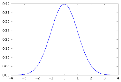 |
| Figure 9. Normal distribution curve |
The normal distribution curve looks like a bell, and simply in KDE we call this as Kernel Shape. If we look at heatmap plugin, there are some Kernel shapes available, there are: Quartic, Triangular, Uniform and Epanechnikov. But there are more kernel shapes available like Cosine, Gaussian, Tricube, etc. Some of these shapes can be seen in figure 10.
Next question. How those shapes are used in estimation of unknown point? As we already knew, the density value is defined by a Kernel shape with a function . To apply it for a heatmap, the function must be transformed into a "geospatial sense" form, because it will be used to predict an unknown value at a point from a point with known value. Here the distance between known to unknown point is a parameter which must be involved in the function. But where we will put it in the function? For example, in the normal distribution function in equation 1, we can see there is (𝚡-𝜇) term. This term is the distance between a value (x) with the expected value (𝜇). This term can be translated as the distance between known to unknown point (d). Then 𝜎 is standard deviation. Standard deviation in statistics measures variation of dataset values. Actually it is the average distance of x to 𝜇. So this term in KDE is translated into bandwidth (h). For Gaussian, h remains as standard deviation but for other kernels h is radius. Hence the equation of KDE with Gaussian Kernel shape has the form as in equation 2, with the visual illustration can be seen in figure 11. If we standardize the h parameter into 1 (100%), the equation 2 can be simplified into equation 3.
 |
| Equation 2. Gaussian KDE function |
 |
| Equation 3. Standardize Gaussian KDE Function |
 |
| Figure 11. Gaussian Kernel Shape |
From figure 11 we can observe that the density value of unknown point will decrease smoothly following the Gaussian Probability Density Function (PDF). It means the unknown value will deviate largely as it moves away from a known point. Other Kernel Shape functions are summarized in the following table.
| Kernel | Function | Shape |
Gaussian
|
|
|
| Quartic |
|
|
| Epanechnikov |
|
|
| Triangular |
|
|
| Triweight |
|
|
| Uniform |
|
|
How to Choose A "Right" Kernel Shape
This is the hardest part in this post. How to choose a right kernel shape? Honestly I don't know the exact answer. But after some research I found a hint in determining a kernel shape. Based on Crimestat III workbook, there are two questions to answer in deciding a kernel shape. First. How large an area will have the effect from an incidents. Second. How much of the effect will remain at original location and how much will be dispersed throughout the bandwidth interval. For example if you think the effect of accident will decrease in linear pattern from an original location, then Triangular Kernel would be a good option. Otherwise if the accident will have the same effect throughout a specified radius, the Uniform kernel would be a good option. So understanding the two questions above for a case will give a better decision in choosing a kernel shape and related parameters.
The following table gives kernel shape option for some types of crime. Although it is for crime mapping, hopefully it could give the idea in defining a kernel shape for other cases. The table was taken from Crimestat III workbook.
I hope this post could give you an understanding what is a Kernel Density Estimation and its application in creating a heatmap. In the
next post, I give a numerical example how this algorithm is used to estimate an unknown value from a reference point. So you will get a complete understanding from theory and its implementation.
Geoanalytics
QGIS
Tutorial


